>
> |
| META TOPICPARENT |
name="CourseExercises" |
Digital Temperature Measurement with the DS18B20
Goal:
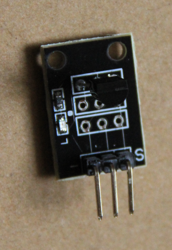
The DS18B20  is a high precision temperature sensor, which already converts the measured analogue temperature into digital values. It uses Maxims 1-wire protocol to speak to its controller, which in our case is the Raspberry Pi. Linux, the Pis operating system, already provides a device driver for this chip, which makes its readout not too complex. In this exercise we will learn how to install a device driver module into the system, see which modules are installed and learn how to interact with the driver through the /sys pseudo file system. is a high precision temperature sensor, which already converts the measured analogue temperature into digital values. It uses Maxims 1-wire protocol to speak to its controller, which in our case is the Raspberry Pi. Linux, the Pis operating system, already provides a device driver for this chip, which makes its readout not too complex. In this exercise we will learn how to install a device driver module into the system, see which modules are installed and learn how to interact with the driver through the /sys pseudo file system.
 |
 |
| DS18B20 |
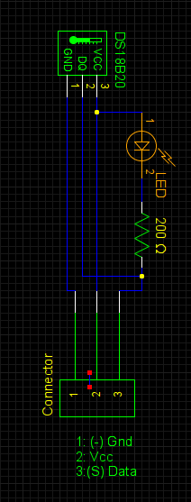
Schematics of the
circuit board |
The DS18B20 and the circuit diagram of its board.
Exercise 1: Setting up the device driver and check that the 1-wire device is seen by the system
Have a look what the commands modprobe, insmod, lsmod and rmmod do. Which kernel modules are loaded and which ones we need in addition. Dont hesitate to look things up on the WEB.
Exercise 2: Read the temperature every 10 s and write it to a file
Read out the DS18B20every 10s, print the results on the screen and write the the results in ASCII format onto a file. The program will be ended by ^C. Catch the corresponding Linux signal and close the file in an orderly fashion before exiting the program.
Exercise 3: Analyze the data
Have the program run for a few hours. Pick up the data file and plot it using gnuplot. You will see that the data jump by fixed values. These fixed values will tell you something about the resolution of the device. What is the resolution?
Knowing that the DS18B20 uses 2s complement representation with 0 corresponding to 0 degrees C and the temperature range is -55 degree C to +125 degrees C, how can you calculate the number of bits needed to represent this range with the resolution determined above?
Exercise 4: Smoothing the data
Implement a moving average filter, averaging over 10 samples and write the result of a second ASCII file. Plot the smoothed data with gnuplot. Then generalize the filter such that the name of the input file, the number of samples used for averaging and a help option can be given to the program as input: e.g. movingAvrg -l 50 -i rawData.txt would calculate the moving average over 50 samples. The data are read from file rawData.txt. The name of the output file is generated from the input file name by appending -smoothed before the extension. In the example it would therefore be called: rawData-smoothed.txt. Have a look at the getopt_long library call on how to handle command line options.
What is a moving average filter?
In our example above we would sum the first 50 (1 .. 49 inclusive) values and divide the sum by 50. This results in our first smoothed data point. Then the first sample is dropped but sample 50 is added and we calculate the average over sample 2..50. This gives us the second data point. The we do the same thing with samples 3..51 and so on. The result is a low pass filter we call moving average filter for obvious reasons.
--  Uli Raich - 2017-04-06 Uli Raich - 2017-04-06
Comments
| META FILEATTACHMENT |
attachment="ds18b20Circuit.png" attr="" comment="" date="1491473054" name="ds18b20Circuit.png" path="ds18b20Circuit.png" size="11574" user="uli" version="1" |
| META FILEATTACHMENT |
attachment="ds18b20.png" attr="" comment="" date="1491473060" name="ds18b20.png" path="ds18b20.png" size="716582" user="uli" version="1" |
|


